Heejo Lee *,
Jong Kim *,
Sung Je Hong*, Sunggu Lee**
*Dept. of Computer Science and Engineering
**Dept. of Electrical Engineering
Pohang University of Science and Technology
San 31 Hyoja Dong, Pohang 790-784, KOREA
1 December 1999
heejo@postech.ac.kr
The recent advanced methods for sparse Cholesky factorization are based on the use of the 2-D block Cholesky to process non-zero blocks using Level 3 Basic Linear Algebra Subprograms (BLAS) [5,6]. Such a 2-D decomposition is more scalable than a 1-D decomposition and has an increased degree of concurrency [23,24]. Also, the 2-D decomposition allows us to use efficient computation kernels such as Level 3 BLAS so that caching performance is improved [19]. Even in a single processor system, block factorizations are performed efficiently [15].
There are few works reported for the 2-D block Cholesky in a distributed-memory system. Rothberg and Gupta introduced the block fan-out algorithm [20]. Similarly, Dumitrescu et al. introduced the block fan-in algorithm [8]. Gupta, Karypis, and Kumar [12] also used 2-D mapping for implementing a multifrontal method. In [18], Rothberg has shown that a block fan-out algorithm using the 2-D decomposition outperforms a panel multifrontal method using 1-D decomposition. Even though the block fan-out algorithm increases the concurrency with reduced communication volumes, the performance achieved is not satisfactory due to load imbalance among the processors. Therefore, several load balance heuristics have been proposed in [21].
However, the load balance is not the sole key parameter for improving the performance of parallel block sparse Cholesky factorization. The load balancing mapping only guarantees that the computation is well distributed among processors; it does not guarantee that the computation is well scheduled when considering the communication requirements. Thus, communication dependencies among blocks may cause some processors to wait even with balanced loads.
In this paper, we introduce a task scheduling method using a DAG-based task graph, which represents the behavior of block sparse Cholesky factorization with the exact amount of computation and communication cost. As we will show in Section 3, a task graph for sparse Cholesky factorization is different from a conventional parallel task graph. Hence we propose a new heuristic algorithm which attempts to minimize the completion time while preserving the earliest start time of each task in a graph. It has been reported that a limitation on memory space can affect the performance [26]. But we do not consider the memory space limitations, since we assume that the factorization is done on a distributed-memory system with sufficient memory to handle the work assigned to each processor. Even though there has been an effort to use DAG-based scheduling for irregular computations on a parallel system with a low-overhead communication mechanism [9], this paper presents the first work that deals with the entire framework of applying a scheduling approach for block-oriented sparse Cholesky factorization in a distributed system.
The next section describes the block fan-out method for parallel sparse Cholesky factorization. In Section 3, the sparse Cholesky factorization is modeled as a DAG-based task graph, and the characteristics of a task for this problem are summarized. Since the characteristics of this type of task are different from the conventional precedence-constrained parallel task, a new task scheduling algorithm is proposed in Section 4. The performance of the proposed scheduling algorithm is compared with the previous processor mapping methods using experiments on the Fujitsu AP1000+ parallel system in Section 5. Finally, in Section 6, we summarize and conclude the paper.
The performance of the factorization is improved by supernode amalgamation, in which small supernodes are amalgamated into bigger ones in order to reduce the overhead for managing small supernodes and to improve caching performance [1,2,20]. Supernode amalgamation is a process of identifying locations of zero elements that would produce larger supernodes if they were treated as non-zeros. In the following, amalgamated supernodes will be assumed by default, and will be referred to simply as supernodes.
In a given ![]() sparse matrix with N supernodes,
the supernodes divide the columns of the matrix (1,..,n)
into contiguous subsets
sparse matrix with N supernodes,
the supernodes divide the columns of the matrix (1,..,n)
into contiguous subsets
![]() .
The size of the i-th supernode is ni, i.e.,
ni=pi+1-pi and
.
The size of the i-th supernode is ni, i.e.,
ni=pi+1-pi and
![]() .
A partitioning of rows and columns using supernodes
produces blocks such that a block Li,j is the sub-matrix
decomposed by supernode i and supernode j.
Then, the row numbers of elements in Li,j are in
.
A partitioning of rows and columns using supernodes
produces blocks such that a block Li,j is the sub-matrix
decomposed by supernode i and supernode j.
Then, the row numbers of elements in Li,j are in
![]() ,
and the column numbers of elements in Li,j are in
,
and the column numbers of elements in Li,j are in
![]() .
.
After the block decomposition of the sparse factor matrix, the total number of blocks is N(N+1)/2. The number of diagonal blocks is N, and all diagonal blocks are non-zero blocks. Each of the N(N-1)/2 rectangular blocks is either a zero block or a non-zero block. A zero block refers to a block whose elements are all zeros, and a non-zero block refers to a block that has at least one non-zero element.
After block decomposition using supernodes, the resulting structure is quite regular [20]. Each block has a very simple non-zero structure in which all rows in a non-zero block are dense and blocks share common boundaries. Therefore, the factorization can be represented in a simple form.
The sequential algorithm for block Cholesky factorization, as described in [20], is shown in Figure 1. The algorithm works with the blocks decomposed by supernodes to retain as much efficiency as possible in block computation. The block computations can be done using efficient matrix-matrix operation packages such as Level 3 BLAS [4]. Such block computations require no indirect addressing, which leads to enhanced caching performance and close to peak performance on modern computer architectures [5].
Let us denote the dense Cholesky factorization of a diagonal block Lkk(Step 2 in Figure 1) as bfact(k). Similarly, let us denote the operation of Step 4 as bdiv(i,k), and the operation of Step 7 as bmod(i,j,k). These three block operations are the primitive operations used in block factorization.
Even though a non-zero block has a sparse structure, we handle it as a dense structure. Since the blocks decomposed by supernodes are well-organized, such a sparse operation for blocks are rarely required [18]. Therefore, we assume that all block operations are handled with dense matrix operations.
For bfact(k), an efficient dense Cholesky factorization can be used,
and bdiv(i,k) and
bmod(i,j,k) are supported by the level 3 BLAS routines
such as ![]() and
and ![]() .
Therefore, we can measure
the total number of operations required for each block operation
as follows [5].
.
Therefore, we can measure
the total number of operations required for each block operation
as follows [5].

The number of required block updates for block Li,j can
be measured. We use the notation
![]() to
denote whether Li,j is a non-zero block or not.
to
denote whether Li,j is a non-zero block or not.
Let
nmod(Li,j) denote the number of required bmod() updates
for Li,j.
When Li,j is a rectangular block,


If a rectangular block Li,j requires m block updates, i.e., nmod(Li,j)=m, then the corresponding task consists of m+1 subtasks including the subtask for the bdiv(i,j) operation. The task has 2m+1 parents as shown in Figure 3. Let us refer to the 2m+1 parent blocks as Li,k0,Lj,k0, ..,Li,km-1, Lj,km-1, Lj,j. A subtask for a block update bmod(i,j,k) executes after the two parent tasks for Li,k and Lj,khave completed and sent their blocks to Li,j. Also, for a diagonal block Lj,j, only one parent for Lj,k needs to be completed before executing the bmod(j,j,k) operation.
Let us assume that there are v non-zero blocks in the
decomposed factor matrix. Each block is represented as
a single task, so that there are v tasks
T1,..,Tv and

Block Cholesky factorization is represented as a DAG,
G=(V,E,W,C). V is a set of tasks
![]() and |V| = v. E is a set of communication edges among tasks,
and |E| = e. Wx, where
and |V| = v. E is a set of communication edges among tasks,
and |E| = e. Wx, where ![]() ,
represents the computation cost
of Tx. If Tx is a task corresponding to a diagonal block Lj,j,
then
,
represents the computation cost
of Tx. If Tx is a task corresponding to a diagonal block Lj,j,
then


We let parent(x) denote the set of immediate predecessors
of Tx, and child(x) denote the set of immediate successors of Tx.
Generally, the task graph G has multiple entry nodes and a single exit node. When a task consists of multiple subtasks, some of them can be executed as soon as the data is ready from the parents of the task. Thus, the time from start to finish for a task Txis not a fixed value, e.g., Wx, but rather depends on the time when the required blocks for subtasks are ready from their parents. Therefore, scheduling a task as a run-to-completion task would result in an inefficient schedule. Most previous DAG-based task scheduling algorithms assume that a task is started after all parent tasks have been finished.
There are two approaches to resolve this situation. One is designing a task model including subtasks. The other is using a block dependency DAG. The former is a complicated approach because the task model may have many subtasks and some of them may already be clustered. This task model is also difficult to handle by a scheduling algorithm. The latter uses a simple, precise task graph as a block dependency DAG. But we can also extract relevant information on all subtasks from the relations in a block dependency graph. Therefore, we devise a task scheduling algorithm using a block dependency DAG.
The proposed scheduling algorithm consists of two stages: task clustering without considering the number of available processors and cluster-to-processor mapping on a given number of processors. Most of the existing algorithms for a weighted DAG also use such a framework [28]. The goal of the proposed clustering algorithm, called early-start clustering, is to preserve the earliest possible start time of a task without reducing the degree of concurrency in the block dependency DAG. The proposed cluster mapping to processors, called affined cluster mapping, tries to reduce the communication overhead and balance loads among processors.
Work and Parents of Subtasks:
A task Ti requiring mi block updates consists of
mi+1 subtasks.
We refer the work for the mi+1 subtasks as
Wi,0,Wi,1,..,Wi,mi. Then the following equation is satisfied:

Earliest Start Time of a Task:
The earliest start time of a task is defined as the earliest time
when one of its subtasks is ready to run.
Note that the earliest start time of
a task is not the time when all required blocks for the task
are received from the parent tasks, although this time has been used by
general DAG-based task scheduling algorithms.
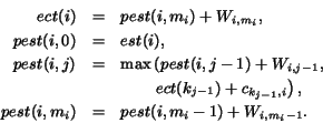
The earliest start time of Ti, est(i), is defined recursively
using the earliest completion time of the parent tasks.
If Ti is the task for a diagonal block, then
est(i) =

When Ti is clustered with a parent Tk, then we can omit the communication cost from Tk to Tiby setting ck,i=0. Thus, the above equations can be used in all of the clustering steps.
Earliest Completion Time of a Task:
The earliest completion time of Ti, referred to as ect(i), is
the earliest possible completion time of all subtasks in Ti.
To define ect(i), we use pest(i,j), which represents
the earliest start time of j-th subtask (
![]() ).
If Ti is the task for a diagonal block, then
).
If Ti is the task for a diagonal block, then

Level of a Task:
The level of Ti is the length of the longest path from Tito the exit task, including the communication costs along that path.
The level of Ti corresponds to the worst-case remaining time of Ti.
The level is used for the priority of Ti in task clustering.
Level is defined as follows.
The proposed early-start clustering (ESC) algorithm reduces the total completion time of all tasks by preserving the earliest start time of each task. ESC uses the level of a task as its priority so that a task on the critical path of a block dependency DAG can be examined earlier than other tasks. Each task is allowed to be clustered with only one of its children to preserve maximum parallelism.
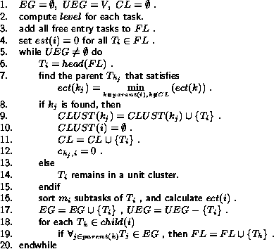
The ESC algorithm uses the lists EG, UEG, CL, and FL. EG contains the examined tasks. UEG is for unexamined tasks. CL is a list of the tasks clustered with one of its children so that a task in CL cannot be clustered with other children. FL is a list of all free tasks maintained by a priority queue in UEG so that the highest level task can be examined earlier than others. CLUST(Ti) refers to the cluster for task Ti. The complete ESC algorithm is described in Figure 6.

The time complexity of ESC is as follows.
To calculate the levels of tasks in Step 2,
tasks are visited in post-order,
and all edges are examined. Hence,
the complexity of Step 2 is O(e).
In the while loop, the most time consuming part is
the calculation of ect(i) in Step 16, which sorts all subtasks
with respect to the ready time of each subtask.
Since the number of subtasks in a task is not larger than
N, sorting of subtasks takes
![]() time.
The complexity of Step 16 is
time.
The complexity of Step 16 is
![]() for v iterations.
Thus, the overall complexity of the ESC algorithm is
for v iterations.
Thus, the overall complexity of the ESC algorithm is
![]() .
.
The most common cluster mapping method is based on a work profiling method [10,17,27], which is designed only for load balancing based on the work required for each cluster. However, by considering the required communication costs and preserving parallelism whenever possible, we can further improve the performance of block Cholesky factorization.
We introduce the affined cluster mapping (ACM) algorithm, which uses the affinity as well as the work required for a cluster. The affinity of a cluster to a processor is defined as the sum of the communication costs required when the cluster is mapped to other processors. We classify the types of unmapped clusters into affined clusters, free clusters, and the heaviest cluster.
ACM finds the processor with the minimum amount of work, and allocates a cluster found by the search sequence. (The cluster with the highest affinity among affined clusters to the processor, or the heaviest cluster among free clusters, or the heaviest cluster among all unmapped clusters.) Initially, all processors have no tasks. Therefore, the heaviest free cluster is allocated first. If the processor with the minimum work has some clusters already allocated, then ACM checks whether there are affined clusters with the processor. If not, ACM checks free clusters. If there are no affined or free clusters, then the heaviest cluster among unmapped clusters is allocated to the processor.
The ACM algorithm uses the lists CLUST, MC, UMC, and FC.
CLUST means the entire set of clusters,
and
CLUST(Ti) represents the cluster
containing task Ti. MC is a list of the mapped clusters, and
UMC is a list of the unmapped clusters. Thus
![]() .
FC is a list of the free clusters. UMC and FC are maintained as
priority queues with the heaviest cluster first.
Each cluster has a list of affinity values for all processors.
The complete ACM algorithm is described in Figure 7.
.
FC is a list of the free clusters. UMC and FC are maintained as
priority queues with the heaviest cluster first.
Each cluster has a list of affinity values for all processors.
The complete ACM algorithm is described in Figure 7.
The time complexity of ACM is analyzed as follows.
Let P denote the number of processors.
Since the number of cluster is less than the number of
tasks, the number of cluster is bounded by O(v).
In Steps 3![]() 5, O(v P) time is required for initialization.
In the while loop, Step 7 takes O(P) time
and Step 8 takes O(v) time;
since the loop iterates for each cluster,
these two steps take O(v2+vP) time.
Steps 14
5, O(v P) time is required for initialization.
In the while loop, Step 7 takes O(P) time
and Step 8 takes O(v) time;
since the loop iterates for each cluster,
these two steps take O(v2+vP) time.
Steps 14 ![]() 20 are for updating
the affinity values for each unmapped cluster
communicating with the current cluster.
In the worst case, all edges are traced twice during the whole loop,
for checking parents and for checking children.
Therefore, the complexity for updating affinities is O(2e).
The overall complexity of the ACM algorithm is thus
O(vP+v2+e).
20 are for updating
the affinity values for each unmapped cluster
communicating with the current cluster.
In the worst case, all edges are traced twice during the whole loop,
for checking parents and for checking children.
Therefore, the complexity for updating affinities is O(2e).
The overall complexity of the ACM algorithm is thus
O(vP+v2+e).
The performance of the proposed scheduling method is compared with various mapping methods. The methods used for comparison are as follows.
The test sparse matrices are taken from the Harwell-Boeing matrix collection [7], which is widely used for evaluating sparse matrix algorithms. All matrices are ordered using the multiple minimum degree ordering [14], which is the best ordering method for general or unstructured problems. Supernode amalgamation [2] is applied to the ordered matrices to improve the efficiency of block operations.
The parallel block fan-out method [20] is implemented on the Fujitsu AP1000+ multicomputer. The AP1000+ system is a distributed-memory MIMD machine with 64 cells. Each cell is a SuperSPARC processor with 64MB of main memory. The processors are inter-connected by a torus network with 25MB/sec/port. For the block operations, we used the single processor implementation of BLAS primitives taken from NETLIB. In order to measure communication costs, we use ts=500 and tc=20, which are estimated from the theoretical peak performance and benchmark tests.
The completion times of BCSSTK14 using various methods are shown in Figure 8. As P increases, the proposed method, schedule, performs well compared with the other methods. The completion time of dag does not decrease even though P increases. This is mainly due to the fact that one cluster includes all the tasks in the critical path of a block dependency DAG, and the huge cluster limits the completion time.
Figure 9 shows the load balance for all methods.
The metric of load balance is
The performance comparison of wrap, cyclic, balance, schedule are shown in Figure 10. In the average case, cyclic is 1.9 times faster than wrap. Also, balance and schedule are 2.5 and 2.8 times faster than wrap, respectively. This means that balance takes 31.6% less time than cyclic, and schedule takes 12.0% less time than balance. In the best case, schedule takes 30% less time than balance. Since the experiments have been conducted on a 2-D mesh topology, cyclic and balance can take the full advantage of their algorithmic properties. If experiments were conducted on other topologies, the gap between the performance of the proposed schedule algorithm and that of cyclic and balance would be larger. From the overall comparison, it can be seen that the proposed scheduling algorithm has the best performance.
We introduced a task scheduling approach for block-oriented sparse Cholesky factorization on a distributed-memory system. The block Cholesky factorization problem is modeled as a block dependency DAG, which represents the execution behavior of 2-D decomposed blocks. Using a block dependency DAG, we proposed a task scheduling algorithm consisting of early-start clustering and affined cluster mapping. Based on experimental results using the Fujitsu AP1000+ multicomputer, we have shown that the proposed scheduling algorithm outperforms previous processor mapping methods. Also, when we applied a previous DAG-based task scheduling algorithm to a block dependency DAG, all tasks in a critical path were clustered into a huge cluster. Thus, the completion time is always bounded by the huge cluster even when the number of processors is increased. However, the proposed scheduling algorithm has good scalability, so that its performance improves progressively as the number of processors increases. The main contribution of this work is the introduction of a task scheduling approach with a refined task graph for sparse block Cholesky factorizations.
This document was generated using the LaTeX2HTML translator Version 98.1p1 release (March 2nd, 1998)
Copyright © 1993, 1994, 1995, 1996, 1997, Nikos Drakos, Computer Based Learning Unit, University of Leeds.
The command line arguments were:
latex2html -split 0 paper.tex.
The translation was initiated by Heejo Lee on 1999-12-01


![\begin{figure}
{\sf\begin{tabbing}
\hspace{0.5cm}\=\hspace{.5cm}\=\hspace{.5cm}\...
...$ {\em affinity}$[p]+c_{k,j}$ . \\
{21.}\> endwhile
\end{tabbing}}
\end{figure}](img41.gif)


