Interactive Evolutionary Algorithm Approach

The problem of simulating ordinary differential equations with fuzzy values, represented by -cut level sets, can be formulated as searching for an overall minimum and an overall maximum curve at each -cut level. Finding a set of initial values and differential equation parameters which represent either the maximum or the minimum of a solution space is impossible, because there exists no such set. An infinite number of problem sets might be necessary to represent the solution space of a differential equation.

The Interactive Evolutionary Algorithm Approach is based on the classical evolutionary algorithm first described by I. Rechenberg [5], [6], and H.P. Schwefel [8]. This model of the evolution is suitable for optimization problems in general, but is not directly suitable for simulating an imprecise ordinary differential equation. The algorithm is called interactive because the objective function assumes that the fuzzy values are interactive during the evaluation of the chromosomes.

One possibility to decode the problem by evolutionary algorithms is by expanding the chromosome to represent the problem set more then once, theoretically infinite size. Then the differential equation solutions represented by these sets build the overall minimum/maximum curve. The drawback of this approach is the increasing number of calculations necessary.

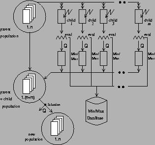
The Interactive Evolutionary Algorithm Approach runs each -cut level and codes the parameters and the initial values of the differential equation just once by the chromosome. For each chromosome the differential equation is simulated and the solution space represented by y-t value pairs is stored in a database. The first time the empty database is filled with the first calculated y-t values. Later the calculated values are saved when they are smaller/bigger than the actual minimum/maximum value stored in the database. When no single problem set of initial values and differential equation parameters exists, the Interactive Evolutionary Algorithm Approach jumps from one possible problem set to the other recording the overall minimum/maximum value in the database.

  

Figure 1: Interactive Evolutionary Algorithm Approach

Fig. 1 visualizes the principle of the approach taken in this work using the graphical notation developed by Rechenberg [6]. From an initial population; parent population 1..n; m children are generated by making copies from randomly selected parents and mutating them. From m evaluated children the best of the children and the parents are selected to build a new population. The process of generating mutated children from parents and select, the best from both is repeated several generations.

Both the minimum and the maximum should be optimized. Therefore the evolutionary process must run twice for every -cut level. Contrary to the classic evolutionary algorithm is the addition of the database which records the absolute minimum/maximum values of the evaluation process.